Scanning Fabry-Perot Interferometer

We next attempted to observe the Zeeman effect on the 780 nm spectral line of Rubidium. This portion of the lab functioned as an extension onto the classic imaging technique, and involved familiarization with a modern (expensive) scanning Fabry-Perot interferometer. We expected greater experimental accuracy and simpler calculation of energy splitting using this new method.

How does a scanning FP work?

We used the Thorlabs SA200-6A scanning Fabry-Perot in junction with a SA201 Spectrum analyzer.

Though the basic structure is the same as for the etalon, two parallel mirrors reflecting light back and forth to resolve different wavelengths. This occurs as light only passes through the mirrors if the distance between them (d) is an integer multiple of half the wavelength (λ).

However, unlike the etalon, the scanning FP does not maintain the same cavity length. Instead, the cavity length sweeps over and over, using piezoelectric transducers.

As the cavity length changes, it resonates with different wavelengths. Therefore, a source with multiple wavelengths (like a lamp split by the Zeeman effect) will see intensity spikes at different points in the sweep of the cavity.

At the back of the scanning FP, there is a photodiode that measures this intensity. We can therefore see peaks correlated with specific wavelengths, such that the interference condition is separated at that specific mirror separation.

What is contained in this extension?

• Mercury 546.1 –> Rubidium 780 nm
  • Both exhibit the anomalous Zeeman Effect
  • Rubidium is within the compatible wavelength range for the scanning FP
• Fabry-Perot Etalon –> Scanning Fabry-Perot
  • May allow us to not rely as heavily on qualitative judgement in determining splitting
  • Digitized as CSV (easier data analysis)
  • Etalon is older & may have gone misaligned
  • Less sensitive to intensity loss through optical trap

Results

We initially collected data on the Rubidium lamp with and without the external magnetic field, to promising results.

We thought that the change observed pre/post application of magnetic field could potential correlate with some kind of Zeeman effect, however there were a number of oddities with our photodiode shapes. First, we were not seeing the nice, sharp peaks we thought we’d see (as seen in the example above from Physlab). Our peaks were also not correlated with the voltage sweeps. This can be seen in the photo below.

It was only when we switched the trigger mode to AC line trigger, that we realized everything we were seeing was just noise from the wall outlet….

Why were we only getting noise?

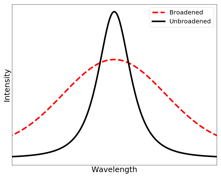
We theorize that our signal was impacted by two sources: doppler broadening and limited FSR.

Doppler Broadening

Doppler broadening is the widening of spectral lines according to temperature. As our Rubidium lamp was quite hot, we might be able to assume some loss of peak resolution occurred due to doppler broadening. For a very sensitive (see section below on FSR) system, the impact of this is magnified.

FSR

For all scanning FP devices, the measurement capabilities are limited by something known as a free spectral range (FSR). Because resonant modes repeat by integer multiples, a single wavelength intensity will correlate with a repeating series of peaks as the cavity scans. The FSR is the distance in wavelength/frequency between those repeating peaks.

In a practical sense, the FSR represents the largest difference in wavelength/frequency that the device can measure before results become ambiguous. Analogously, if you have a repeating ruler that reads 0-10in, and try to measure a difference of 12in, your measurement will be confused as 2in. In the same sense, we cannot measure frequency differences (frequency is the standard unit for FSR) above 1.5GHz.

After some quick calculations we found that the FSR of 1.5GHz was not compatible with our system at all.

We started by recognizing that we are constrained by minimum resolvable, and maximum achievable magnetic fields in the range of roughly 100G to 15,000G. The magnetic field necessary to introduce a frequency shift equal to one free spectral range is:

B_FSR = hc/2d * 2m_e/ℏgeΔm_j = 2πm_ec/edgΔm_j

Therefore, we require 100G =< B_FSR =< 15,000G. Translating this to FSR in frequency provides that our FSR in frequency is bounded by 0.14-21 GHz.

While the small free spectral range of the scanning cavity interferometer is technically within the bounds, a successful measurement under these conditions will require a very narrowband source. As the scanning FP is designed to work with a laser, and accounting for the effects of doppler broadening, we this is not compatible. Additionally, the B_FSR will occur at a very small field, so the field-dependent emission line must be very narrow or else its power will be spread over most or all of the free spectral range.

Future work might benefit from using an interferometer with a free spectral range of FSR=5-10 GHz (i.e., spacing d = 15-30 mm). In this case, a maximum magnetic field of 15,000 G would be sufficient to shift the field-dependent lines by 2-4 free spectral ranges, while still allowing for relatively broad emission lines.