We first observed the Zeeman effect on the 546.1 nm spectral line of mercury. We were not able to achieve enough resolution to measure the splitting, but we were able to visually see the Zeeman effect and create a rough estimate of the Landé factor.
The Method
For observing the 546 nm emission line in mercury, we used a mercury spectral lamp. Mercury, as with any atom, has numerous spectral lines. A 546 nm filter can be inserted in the optical pathway prior to the imaging to isolate the 546 nm line.
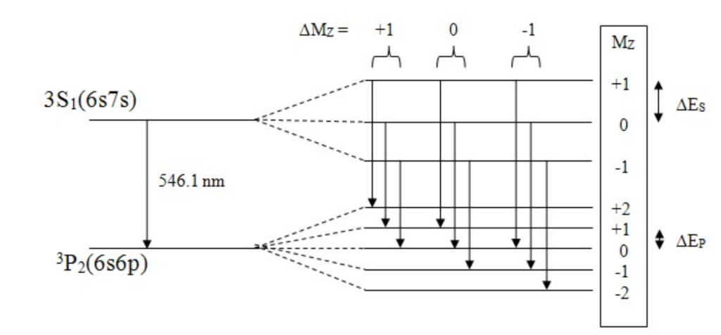
In the presence of a magnetic field, the 546 nm line splits into three lines (assuming you only look at the π polarized lines). The technical details of the polarization of the Zeeman lines has been omitted on this website, but can be easily found in any undergraduate quantum mechanics textbook, such as in A Modern Approach to Quantum Mechanics by Townsend.
The wavelength difference between these lines can be determined by sending emitted light through a Fabry-Perot etalon. A guide to the Fabry-Perot etalon is provided in the drop-down menu below. I highly recommend that you read it; we will be referencing the content in this section numerous times throughout the website. Light that passes through the etalon forms a series of concentric rings, as shown in the Figure 1. The separation of these rings can be used to determine the wavelength differences.
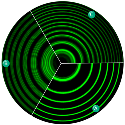
Mercury is known for having bright, spaced out (in wavelength) spectral lines.
One line is particularly easy to observe! This line is the green line at 546.1 nm.
Not only is it in the visible range for humans (meaning we don’t have to rely purely on a detector to be able to observe it), but it also produces a clean triplet of lines with equal spacing under the Zeeman Effect. This makes the splitting straightforward to measure and observe.
This particular line has become a bit of a “standard” for Zeeman Effect experiments involving Fabry-Perot interferometry.
A Fabry-Perot (FP) etalon is comprised of two highly-reflective flat mirrors that are perfectly parallel to one another and separated by length l.

Consider a single ray of monochromatic light at wavelength λ. Monochromatic light incident on the FP will reflect numerous times between the two mirrors. At every point of reflection (see points b and c on the diagram), a small fraction of light is also transmitted since the mirrors are not perfectly reflective. Rays of transmitted light then interfere with each other outside of the etalon. At certain angles, light constructively interferes, while at other angles, light destructively interferes. Since light enters the etalon at a variety of angles, the resulting interference pattern is a series of concentric rings (see Figure 1) described by
where n is an integer and d is the distance between the two mirrors (I have replaced l with d by convention). Note: The n = 0 order of light actually corresponds to the largest diameter ring, since cos(90) = 0! This differs from the convention used for diffraction gratings, where n = 0 corresponds to the center fringe.
Now imagine a light source that contains many different wavelengths of light. From equation (1), we see that the spacing between concentric rings is different for different wavelengths of light. For example, rings of red light (∼600 nm) will be spaced closer together than rings of green light (∼500nm), since the cosθ term is larger for red light (remember larger cosθ corresponds to smaller θ).
At a certain Δλ in wavelength, the mth order of longer wavelength light overlaps with the (m+1)th order of shorter wavelength light. Δλ is known as the free spectral range (FSR) of the etalon, and is given by
FSR can be equivalently though of as the wavelength difference between two adjacent bright rings in the interference pattern. It is important that the FSR of an etalon is large enough such that it can resolve the Zeeman splitting of the mercury spectral line. If the splitting is larger than the FSR, rings of different wavelengths begin to overlap, making an accurate measurement of the splitting almost impossible. The free spectral range is often given in terms of the frequency of light as opposed to its wavelength.
Derivations of equations (2) and (3) are provided on pages 414 – 425 of Optics (4th ed.) by Hecht.
Lastly, we would like include some questions we had and answered while learning about the Fabry-Perot etalon.
- The light emitted by the mercury lamp is not in randomly phased. Does the light entering a Fabry-Perot have to be coherent (every photon in phase)?
No! It would seem that light entering the etalon would have to be coherent in order for the light to then interfere constructively outside of the etalon. After all, if the light was randomly phased, how would we get consistent areas of destructive and constructive interference? But remember that the interfering rays are simply many transmitted rays originating from the same incident ray, as shown in Figure 2. Therefore, at angles of constructive interference, all transmitted rays are perfectly in phase, since they all originated from the same incident ray.
- Fabry-Perot etalons are manufactured to only work within a certain wavelength range. Why is this the case?
Mirrors are fabricated to only be high-reflective in certain wavelength ranges. Therefore, if you wanted to image a different source, say Rubidium which emits mostly infrared light, you would need to use a different etalon with different mirrors.
Experimental Setup
Materials
- Electromagnet
- Mercury Pen Lamp
- 20 cm focal length biconvex lens
- 30 cm focal length biconvex lens
- 546nm filter
- Fabry Perot etalon (mirror spacing of 5.71 mm)
- Nikon J1 Camera (with focus set to infinity)
Optical Setup
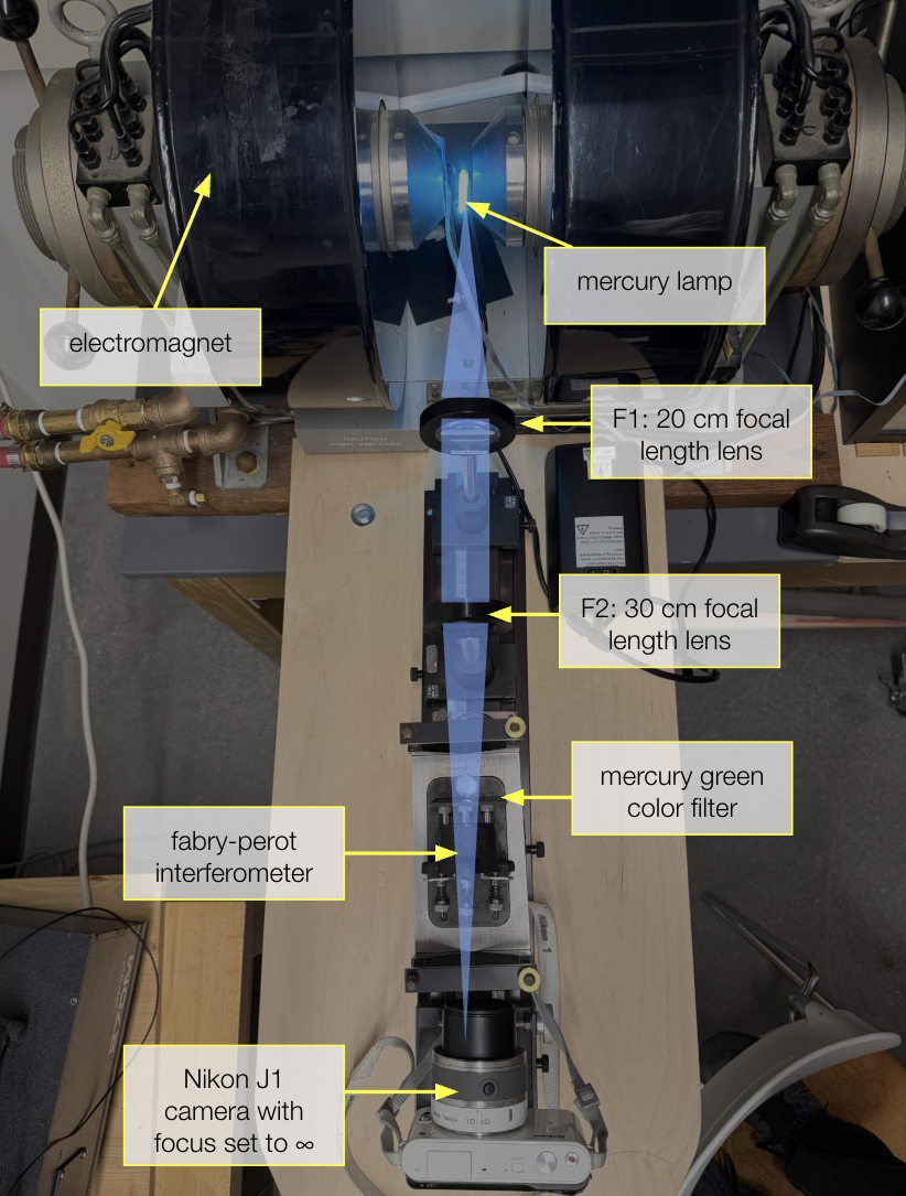
Positioning the Lenses
All components are mounted on an a rail to ensure axial alignment. The first lens, F1, is exactly exactly one focal length (20 cm) away from the mercury lamp. This lens collimates the diverging light emitted from the lamp.
Since our camera focus was set to infinity, the camera’s lens would have focused this collimated light onto the camera chip, producing an unwanted image of the lamp. We don’t want to image the lamp itself. We want to image our interference pattern, and we want this pattern to be set against a background of diffuse light (think a big blurry splotch of light) to ensure maximal contrast between the bright rings and the dark areas in between.
Therefore, I placed a second lens of 30 cm roughly one focal length away from the camera. This lens technically focuses the collimated light onto the camera, but since the camera has a lens itself, the final image on the camera chip is unfocused and blurry. We have thus intensional created a blurry and diffuse background for our interference pattern! P.S. I did not choose 30 cm for any particular reason; it was simply what I had available. In fact, this setup can be achieved with any combination of lenses with any focal length.
The Fabry-Perot Etalon
Preferably, a 546 nm filter is placed directly before the Fabry-Perot etalon to only image to 546 line. However, the 546 nm filter available to us also attenuated the intensity of the 546 nm line, resulting in an extremely dim image. We therefore opted for the second best option, which was a green-yellow color filter that unfortunately allowed both the green (546nm) and yellow (577nm and 579nm) lines of mercury through. As a result, we ended up imaging the Zeeman effect in both the yellow and green, resulting in an image nearly impossible to quantitatively analyze.
The Fabry-Perot is positioned parallel to the optical axis directly before the camera. Our etalon has three screws on the back that allows for fine tuning of the mirrors. We assumed the mirrors in the etalon were already parallel and chose not to adjust the screws.
The Camera
The camera was placed on a translational stage that allowed for movement perpendicular to the optical axis. This allowed us to finely tune the position of the camera such that the interference fringes were centered on our image.
The camera’s focus was set to infinity, as stated above, and it’s exposure was set to the longest option of 1/60th of a millisecond. Additionally, we used the furthest optical zoom available.
Procedure
With the green-yellow filter installed (this was the only filter that allowed enough light through to produce an image, see “Aligning the optical pathway” section for reasoning), we took a video of our interference rings at various magnetic field strengths, ranging from 0 to 11,000 Gauss. We had someone turn up current on the electromagnet in increments of 0.2 amps (see Figure NN) and verbally read out the current. This allowed to know exactly what the magnetic field strength was at different times in the video.
Results
As the magnetic field increases, the rings slowly start to wash out. This washing out is the Zeeman effect in action! We are seeing the split lines “filling up” the areas of destructive interference. Unfortunately, we weren’t able to achieve high enough resolution to make out the splitting of the energy levels as shown in Figure 1b. We are essentially seeing a blurry version of figure 1b.
Notice that the rings completely wash out when Nora reads out a current of “1.2 amps” which corresponds to a magnetic field of 8500 Gauss from our calibration curve. The rings then slowly start to appear again as Nora continues to increase the magnetic field strength from 8500 Gauss to its maximum value. We concluded that at 8500 Gauss, the split line perfectly traversed half the distance between two adjacent bright rings, resulting in a washout of the interference pattern. Since the wavelength difference between two adjacent bright rings is the free spectral range of our etalon, a split line at halfway this distance is one half a free spectral range away from the nominal wavelength. Note: Throughout this section, we assumed that we were only looking at the 546 nm line in mercury even though our filter let through the yellow line as well. We were able to make this approximation since our spectrometer data showed that the yellow light was extremely dim compared to our green light.
We used this to determine a rough quantitative estimate of 1.1 for Δgjmj, where gj Landé factor and mj is the quantum number of total angular momentum.
Recall from the Theory section that the change in energy due to the Zeeman effect is
As stated in the “How does the Fabry-Perot etalon work?” section, the frequency difference corresponding to one free spectral range is
In terms of energy, this equation can be rewritten as
where h is Planck’s constant. We can set equation 4 and 6 equal to eachother to solve for Bfsr.
For a transition j to j’, we can quantify Δgjmj = gjmj-gj’mj’.
From our value of Bfsr = 2*8500 = 17000 Gauss, we get
This is a unitless value that describes a specific Zeeman transition in the 546 nm line in mercury. The theoretical value of Δgjmj for each of the nine transitions.
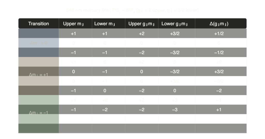
We see that our value for Δgjmj = 1.1 is closest to the theoretical value of +1 or -1 for the transitions from mj = 1 to mj’ = 2 or mj = -1 to mj’ = -2. We can interpret these transitions the brightest or highest intensity transitions.
Leave a Reply